Simulation Manual: Elastic Collision in One Dimension
Are you interested in translating this manual into another language? Please contact me here.
لقراءة النسخة العربية أنقر هنا.
Introduction
This simulation demonstrates the conservation laws in one-dimensional elastic collisions: the law of conservation of linear momentum and the law of conservation of kinetic energy.
When the initial parameters are set (the masses of the balls and their initial velocities), the final velocities can be determined, and you will observe the colliding balls moving accordingly.
Another idea this simulation demonstrates is that the center of mass of an isolated system keeps moving with the same velocity before and after the collision. To show this, there is the option to take successive shots of the center of mass of the system formed by the two balls at equal time intervals, and two draggable vertical markers are provided to measure the distance between successive dot-prints, so you can check that the distances between these successive dot-prints are equal and hence the center of mass covers equal distances during equal time intervals, which means that its velocity is constant.
Click here to run the simulation.
Target Users
This simulation is instrumental and informative for students who want to virtually experiment without the need of a real lab (or in the case of lab equipment shortage).
The simulation is also invaluable and handy for teachers and lab instructors who want to engage their students in performing lab activities on the collisions of elastic objects and draw conclusions and discover the underlying principles.
I advise the instructors who want to benefit from this simulation to introduce the experiment in a directed discovery approach. This way, the students are guided through repeating the experiment to discover the conservation laws mentioned above rather than receiving them.
Importance of the Simulation
The collision experiment is one of the intricate physics experiments. It is usually performed on an air table or on an air track, both of which are expensive and require a lot of preparation and precise measurement. This equipment is not easily found in every school lab. So, this simulation makes it easy for high-school and undergraduate students to perform an affordable activity that enables them to acquire the required skills and knowledge in this topic.
Of course, it is much better to perform a real experiment instead of a virtual experiment when possible. However, the virtual experiment is much appreciated in the case of a shortage of equipment or for a preliminary activity to prepare the students for the real lab.
Instructional designers and course creators may find that this simulation facilitates their work.
Conservation Laws in Collisions
The Law of Conservation of Linear Momentum of an Isolated System
The total linear momentum of an isolated system is conserved (does not vary).
By isolated system, we mean a system formed of two or more particles that may interact with each other but do not interact with any other particles. Since they are not interacting with any other particles, this means that either there is no external force acting on this system, or the external forces on the system cancel each other out so the summation of the external forces is zero. Mathematically, we write the law as follows:
![\[\sum_{}^{}{\overrightarrow{F}}_{\text{ext}} = \overrightarrow{0} \Longrightarrow \sum_{}^{}\overrightarrow{P_{\text{total}}} = \overrightarrow{\text{constant}}\]](https://physics-zone.com/wp-content/ql-cache/quicklatex.com-6e7a6b002b2012671c2b1d0e8933b6bc_l3.svg "Rendered by QuickLaTeX.com")
Where  is the total external force acting on the system,
  is the total linear momentum of the system, and by
  , we mean constant vector.
During collisions, the total linear momentum of the colliding particles is conserved. That means it stays constant before and after a collision. This is true in general even if the colliding particles are submitted to external forces such as the weight or friction (so in this case the system is not isolated). This is because the external forces like the weight of the balls or the friction are negligible compared to the internal impact forces that took place between the particles during the collision. So, as an approximation, the system is considered isolated only during the collision (which lasts for a very short time interval). In this case, we say that the total linear momentum of the system just before the collision and just after the collision is conserved. Mathematically:
![\[\sum_{}^{}{\overrightarrow{F}}_{\text{ext}} = \overrightarrow{0} \Longrightarrow \sum_{}^{}{\overrightarrow{P}}_{\text{before}} = \sum_{}^{}{\overrightarrow{P}}_{\text{after}}\]](https://physics-zone.com/wp-content/ql-cache/quicklatex.com-bc05a5055b309006af1426e4abfdff71_l3.svg "Rendered by QuickLaTeX.com")
In the case of the experiment of this simulation:
![\[{\overrightarrow{P}}_{1\ before} + {\overrightarrow{P}}_{2\ before} = {\overrightarrow{P}}_{1\ after} + {\overrightarrow{P}}_{2\ after}\]](https://physics-zone.com/wp-content/ql-cache/quicklatex.com-f1afde7c145b1cb95cccee92891415f0_l3.svg "Rendered by QuickLaTeX.com")
![\[\Leftrightarrow m_{1} \cdot {\overrightarrow{v}}_{1} + m_{2} \cdot {\overrightarrow{v}}_{2} = m_{1} \cdot {{\overrightarrow{v}}^{'}}_{1} + m_{2} \cdot {{\overrightarrow{v}}^{'}}_{2}\]](https://physics-zone.com/wp-content/ql-cache/quicklatex.com-13532dabdfe890b312fea4157f40c6af_l3.svg "Rendered by QuickLaTeX.com")

Where  and
and  are respectively the initial velocities of ball 1 (of mass m1) and ball 2 (of mass m2), and
  and
and  are respectively the final velocities of ball 1 and ball 2 (from now on, let us call them m1 and m2 for short).
In a one-dimensional collision, the velocity vectors , , , and can be replaced by their algebraic values  ,
,  ,
,  , and
, and  on the x-axis, so:
![\[m_{1} \cdot v_{1} + m_{2} \cdot v_{2} = m_{1} \cdot v_{1}^{'} + m_{2} \cdot v_{2}^{'}\]](https://physics-zone.com/wp-content/ql-cache/quicklatex.com-2c8b1aeafb14c1fa12e1223725246501_l3.svg "Rendered by QuickLaTeX.com")
The Law of Conservation of Kinetic Energy During an Elastic Collision
Furthermore, if during the collision there is no dissipation of energy in the form of heat, permanent deformation of the colliding particles, radiation, etc., then the collision is said to be elastic. In this case, the total kinetic energy of the colliding particles just before and just after the collision is conserved. Mathematically:
![\[Elastic\ collision \Longrightarrow \sum_{}^{}K_{\text{before}} = \sum_{}^{}K_{\text{after}}\]](https://physics-zone.com/wp-content/ql-cache/quicklatex.com-b37e48053d27e79ed7d581adb7258a7e_l3.svg "Rendered by QuickLaTeX.com")
Where Kbefore is the total kinetic energy of the colliding particles just before the collision, and Kafter is the total kinetic energy of the colliding particles just after the collision.
In the case of the experiment of this simulation:
![\[K_{1\ before} + K_{2\ before} = K_{1\ after} + K_{2\ after}\]](https://physics-zone.com/wp-content/ql-cache/quicklatex.com-67964ed295a5c4e63968a8934bb80f73_l3.svg "Rendered by QuickLaTeX.com")
![\[\Leftrightarrow \frac{1}{2}{\cdot m}_{1} \cdot v_{1}^{2} + \frac{1}{2} \cdot m_{2} \cdot v_{2}^{2} = \frac{1}{2} \cdot m_{1} \cdot {v^{'}}_{1}^{2} + \frac{1}{2} \cdot m_{2} \cdot {v^{'}}_{2}^{2}\]](https://physics-zone.com/wp-content/ql-cache/quicklatex.com-6fa5078ba3a5d6ad609285504c033d43_l3.svg "Rendered by QuickLaTeX.com")
Where and are respectively the algebraic values of the initial velocities of m1 and m2, and  and
and  are respectively the algebraic values of the final velocities of m1 and m2.
Elastic Collision
Combining the two conservation laws during an elastic collision, one can determine the final velocities of the two colliding particles of given masses just after the collision if the initial velocities of the two particles just before the collision are known. After some mathematical manipulations of the two equations:
and
![\[\frac{1}{2}{\cdot m}_{1} \cdot v_{1}^{2} + \frac{1}{2} \cdot m_{2} \cdot v_{2}^{2} = \frac{1}{2} \cdot m_{1} \cdot {v^{'}}_{1}^{2} + \frac{1}{2} \cdot m_{2} \cdot {v^{'}}_{2}^{2}\]](https://physics-zone.com/wp-content/ql-cache/quicklatex.com-e6e4c93b880c2e5f2235aae0b19dec37_l3.svg "Rendered by QuickLaTeX.com")
You can find the algebraic values of the final velocities in terms of the masses m1 and m2 and the algebraic values of the initial velocities:
![\[v_{1}^{'} = \frac{m_{1} - m_{2}}{m_{1} + m_{2}}v_{1} + \frac{2m_{2}}{m_{1} + m_{2}}v_{2}\]](https://physics-zone.com/wp-content/ql-cache/quicklatex.com-979fd632c05423efcfc0bbd8a82e6d29_l3.svg "Rendered by QuickLaTeX.com")
![\[v_{2}^{'} = \frac{2m_{1}}{m_{1} + m_{2}}v_{1} + \frac{m_{2} - m_{1}}{m_{1} + m_{2}}v_{2}\]](https://physics-zone.com/wp-content/ql-cache/quicklatex.com-5acd704a4512baf18ca5905bc275eb6c_l3.svg "Rendered by QuickLaTeX.com")
Remarks
In this simulation, you can also check two special cases:
1. If the two particles are of equal masses, then substituting in the above two expressions of the final velocities, we find that the two particles exchange velocities:
![\[m_{1} = m_{2} \Rightarrow v_{1}^{'} = v_{2}\text{\ and\ }v_{2}^{'} = v_{1}\]](https://physics-zone.com/wp-content/ql-cache/quicklatex.com-165dae79bc720cb9f6f1cd74649ef556_l3.svg "Rendered by QuickLaTeX.com")
2. If the two particles are of equal masses and the second particle was initially at rest, they exchange velocities, and hence after the collision, the first particle stops and gives off its velocity to the second particle:
![\[m_{1} = m_{2}\text{\ and\ }v_{2} = 0 \Rightarrow v_{1}^{'} = 0\ and\ v_{2}^{'} = v_{1}\]](https://physics-zone.com/wp-content/ql-cache/quicklatex.com-c7e122a89abf24751465e3844a488129_l3.svg "Rendered by QuickLaTeX.com")
The Motion of the Center of Mass of an Isolated System
The linear momentum of a system of particles of constant mass is equal to that of its center of mass G, where the total mass is assumed to be concentrated at the center of mass. In the case of an isolated system, the linear momentum of the system is constant and hence the velocity of the center of mass G of the system stays constant. Hence, the center of mass of an isolated system moves with uniform speed along a straight line. Mathematically:
![\[{\overrightarrow{P}}_{\text{total}} = M\overrightarrow{V_{G}}\]](https://physics-zone.com/wp-content/ql-cache/quicklatex.com-1bbdd55e4d36804ac2ac689b2d214b3f_l3.svg "Rendered by QuickLaTeX.com")
Where  is the total linear momentum of the system, M is the total mass of the system, and
  is the velocity of the center of mass of the system.
In the case of an isolated system:
![\[{\overrightarrow{P}}_{\text{total}} = \overrightarrow{\text{constant}} \Longrightarrow M\overrightarrow{V_{G}} = \overrightarrow{\text{constant}} \Longrightarrow \overrightarrow{V_{G}} = \overrightarrow{\text{constant}}\]](https://physics-zone.com/wp-content/ql-cache/quicklatex.com-91c80f725e22078af8c0905b7d1e0eb1_l3.svg "Rendered by QuickLaTeX.com")
So, the center of mass G is moving with uniform velocity.
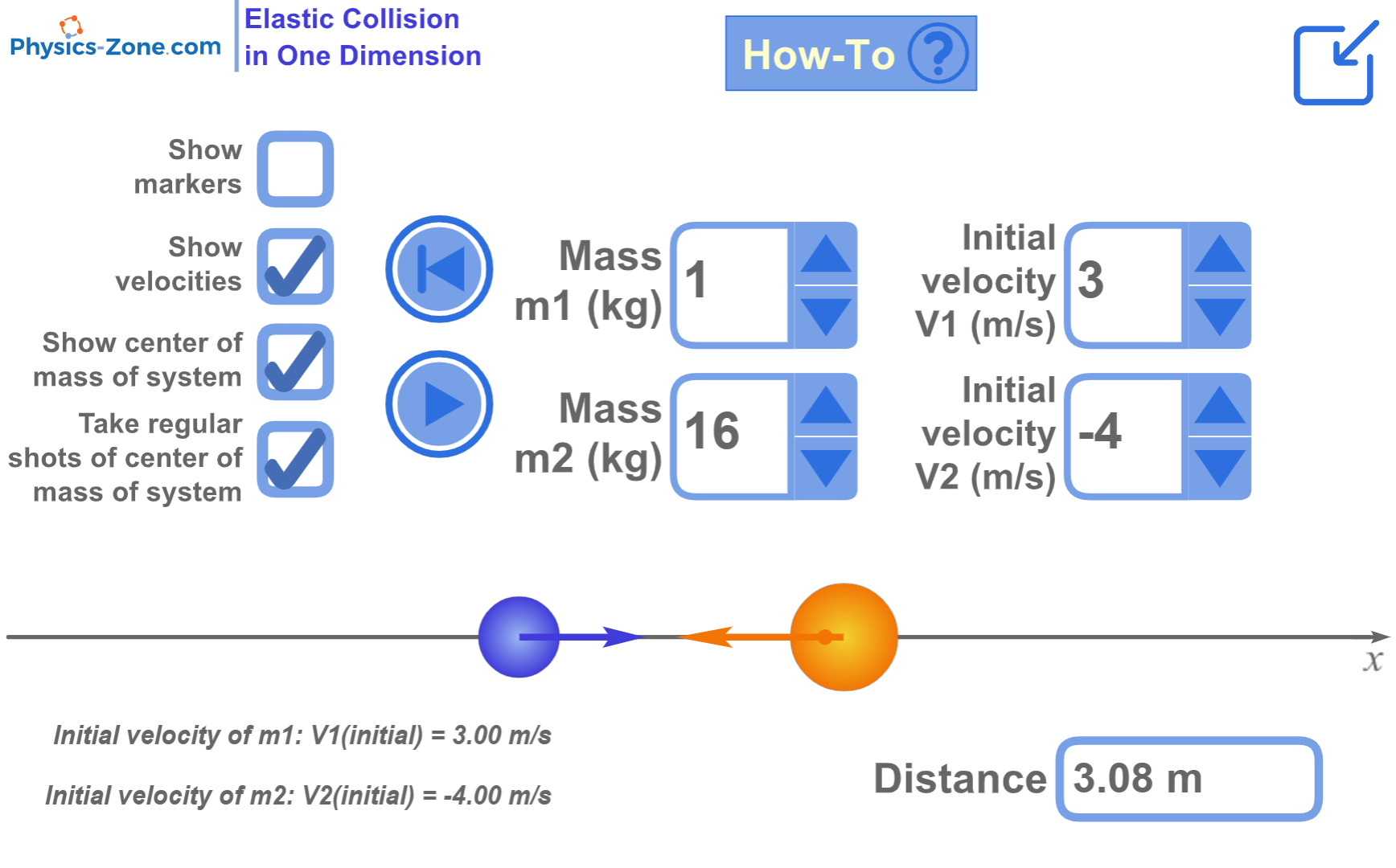
Working Guidelines for the Simulation
In this section, we are going through each element of the simulation and explaining its function.
Maximize / Minimize toggle button: Click this button to enter full-screen mode or to restore the window mode.

m1 and m2: These are the colliding balls of masses m1 and m2 (m1 and m2 are set by the user). When the experiment starts, they will move with velocities also set by the user. Note that they collide elastically, so the law of conservation of linear momentum and the law of conservation of kinetic energy are applied during the collision.
x-axis: This is the axis on which the two balls move. Remember that the experiment is one-dimensional, so each ball will move either to the left or to the right.

Play button: When you finish setting the parameters of the experiment (the masses of the balls m1 and m2, and their velocities V1 and V2), click this button to start the motion of the two balls.

Reset/Stop Button: Click this button to stop the current experiment and bring the two balls to their initial positions, without resetting their masses or velocities.

“Show velocities” check button: Tick this check button to show the velocity vectors on each of the two balls.

“Show center of mass of system” check button: Tick this check button to show the center of mass of the two balls as they move.

“Take regular shots of center of mass of system” check button: Tick this check button to duplicate the center of mass of the two balls on the x-axis periodically (every constant time interval). This shows you that the center of mass covers equal distances every equal time interval.

“Show markers” check button: Tick this check button to enable the visibility of the vertical markers. When you want to measure the distance between two positions on the x-axis, drag these markers and place one of them at one position and the other at the other position, then you will see the distance between these two positions displayed inside the textbox labeled “Distance”.

“Distance” text box: This text box displays the distance between the two markers on the x-axis. This is useful to measure the distance between successive dot-prints of the center of mass of the system formed by the two balls and to prove that they are equally spaced and hence the center of mass moves with uniform velocity.

“Mass m1” stepper button: Use this stepper button to increase or decrease the mass m1 of ball 1 by 1 kg in each step.

“Mass m2” stepper button: Use this stepper button to increase or decrease the mass m2 of ball 2 by 1 kg in each step.

“Initial velocity V1” stepper button: Use this stepper button to increase or decrease the velocity of the ball m1 by 1 m/s in each step. Note that positive velocity means that the ball is moving in the positive direction (to the right), while negative velocity means that the ball is moving in the negative direction (to the left).

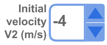
“Initial velocity V2” stepper button: Use this stepper button to increase or decrease the velocity of the ball m2 by 1 m/s in each step. Note that positive velocity means that the ball is moving in the positive direction (to the right), while negative velocity means that the ball is moving in the negative direction (to the left).
“Initial velocity of m1“: Before the collision, this displays the initial velocity of m1.
![]()
“Initial velocity of m2“: Before the collision, this displays the initial velocity of m2.
![]()
“Final velocity of m1“: After the collision, this displays the final velocity of m1.
![]()
“Final velocity of m2“: After the collision, this displays the final velocity of m2.
![]()
Conclusion
With this simulation, which is rich with controls and visuals to illustrate the laws of conservation in the one-dimensional elastic collision, and with the proper instructional methodologies, the instructor will be able to empower the sense of discovery in the learners and introduce the concept of collision in a simple, clear, and visually rich presentation, enabling the learners to acquire the required learning objectives.
The simulation is coded with the latest HTML5/JavaScript web tools.