Simulation Manual: Photoelectric Effect Experiment
Are you interested in translating this manual into another language? Please contact me here.
لقراءة النسخة العربية أنقر هنا.
Introduction to the Simulation
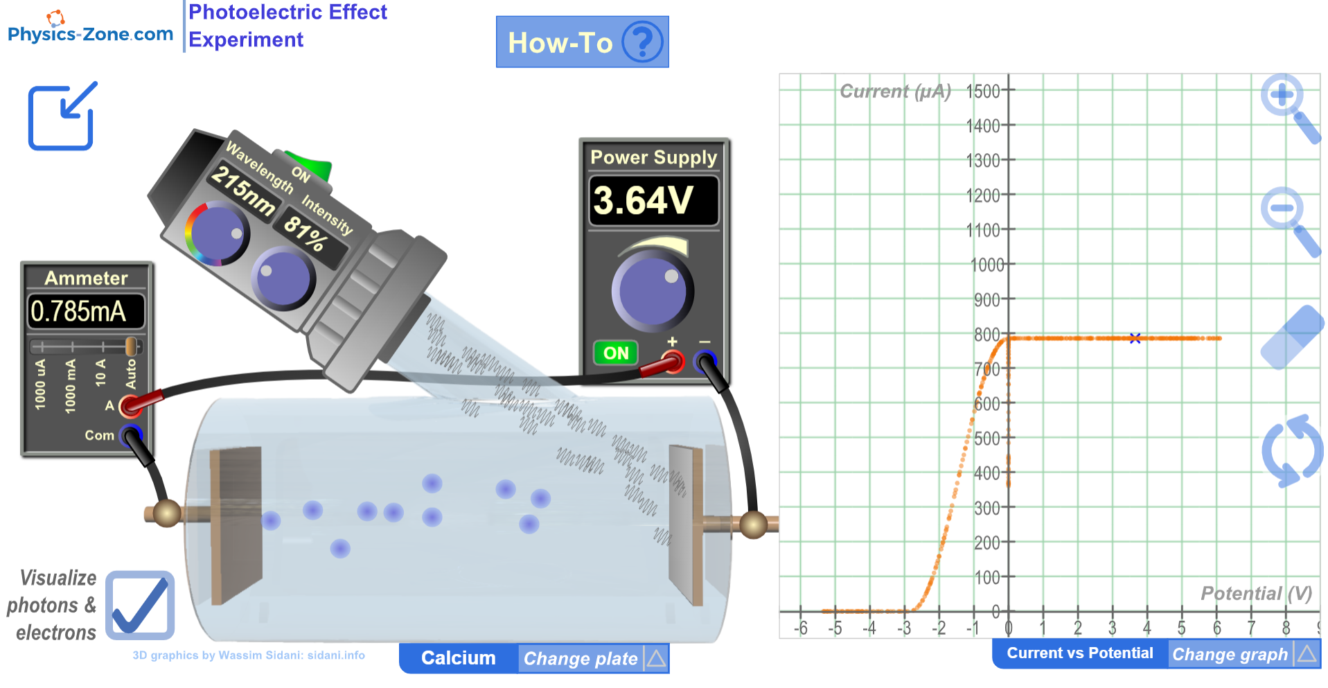
With this comprehensive and realistic-like photoelectric effect experiment simulation, you will be able to illustrate the following:
The variations of the photocurrent versus potential.
The variations of the photocurrent versus light intensity.
The variation of the kinetic energy of the ejected electrons versus the incident light frequency.
It comes with a graph where you can trace each type of variation as you vary the parameters of the experiment.
Plus, you can experiment and discover more with this simulation.
Click here to run the simulation.
Target Users
This simulation is instrumental and informative for students who want to virtually perform the experiment without the need of a real lab (or in the case of lab equipment shortage). They can record measurements of several physical quantities such as the photocurrent, wavelength, voltage, light intensity, etc., and from these results, they can plot the corresponding graphs and calculate other physical quantities such as the work function of the used element or Planck’s constant.
The simulation is also invaluable and handy for teachers and lab instructors who want to engage their students in performing lab activities on the photoelectric effect and draw conclusions and discover the underlying principles.
I advise the instructors who want to benefit from this simulation to introduce the experiment in a directed discovery approach. This way, the students are guided through repeating the experiment to discover the underlying principles rather than receiving them.
Importance of the Simulation
The photoelectric effect experiment is one of the intricate physics experiments. Its equipment is not easily found in every school lab. So, this simulation makes it easy for high-school and undergraduate students to perform an affordable activity that enables them to acquire the required skills and knowledge in this topic.
Of course, it is much better to perform a real experiment instead of a virtual experiment when possible. However, the virtual experiment is much appreciated in the case of a shortage of equipment or for a preliminary activity to prepare the students for the real lab.
Instructional designers and course creators may find that this simulation facilitates their work.
Advantages Over Other Similar Simulations Available on the Internet
If you search the internet for photoelectric effect simulation, you may find a simulation that provides realistic-like results that are good enough to be used in lab reports, but lacks the visuals that give the impression of the lab environment, and most importantly cannot be run without the proper runtime environment as the technology it was designed with is not supported by modern browsers anymore.
You may also find a simulation that illustrates only one aspect of the experiment and hence is not comprehensive. Or you may find other simulations that are not realistic in the way they provide the measurement.
Moreover, you will find a lot of animations that are not interactive — you can only view one aspect of the process.
This simulation, on the other hand, provides the opportunity to engage in a lab environment that looks like the real one. It enables you to interact and vary all the available parameters of the phenomenon and take measurements that are close to the real measurement with a small margin of discrepancy. So high school students can write reliable lab reports for their assignments using this simulation. Moreover, the graph provided in the simulation gives them a deeper insight into the interdependence of the variations of the physical quantities in the experiment.
A Short Introduction to the Photoelectric Effect
The photoelectric effect is the emission of electrons from a material hit by electromagnetic radiation, such as light. These emitted electrons are called photoelectrons.
There is a remarkable observation in the photoelectric effect that cannot be explained by classical physics: there is a threshold frequency, below which no photocurrent is emitted from the plate being hit by the electromagnetic radiation, regardless of the intensity of the light beam or the potential applied across the plates.
To explain experimental data from the photoelectric effect, Albert Einstein published a paper in 1905, advancing the hypothesis that light energy is carried in discrete quantized packets. Einstein theorized that the energy in each quantum of light was equal to the frequency of light multiplied by a constant, later called Planck’s constant. A photon above a threshold frequency has the required energy to eject a single electron, producing the observed effect. This was a key step in the development of quantum mechanics.
This effect has found uses in electronic devices, mainly in light detection and precisely timed electron emission. Other uses include image sensors, photoelectron spectroscopy, and more.
Working Guidelines for the Simulation
In this section, we are going through each element of the simulation and explaining its function.
General Controls
Maximize / Minimize toggle button: Click on this button to enter full-screen mode or to restore the window mode.

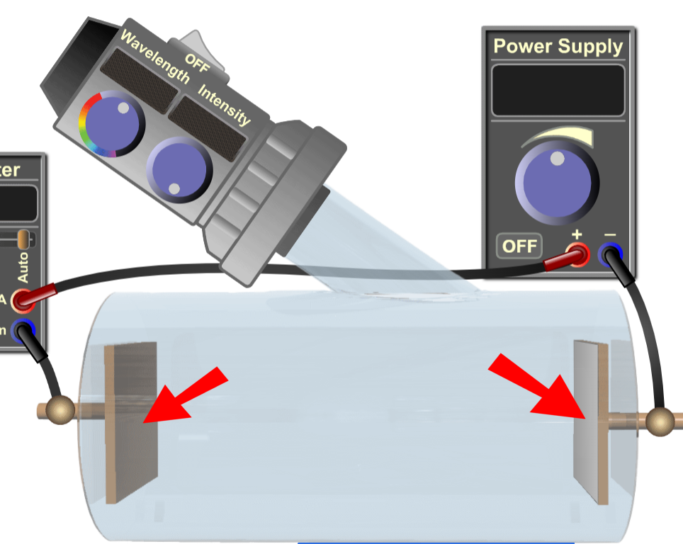
Power Supply
Power Supply: This instrument supplies positive and negative voltage across the plates inside the vacuum tube. Note that you have to turn it on to have current running in the circuit even if there are ejected electrons inside the vacuum tube, since when the power supply is OFF it acts as an open circuit.
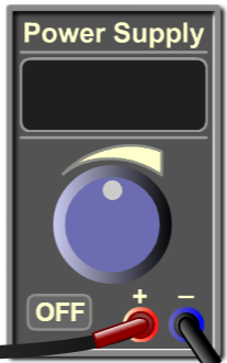
ON/OFF switch: This is used to turn on or off the power supply.
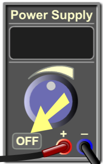
Knob: You can rotate this knob to vary the value of the voltage.
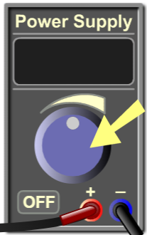
Display: This shows the value of the voltage generated by the power supply in volts.

Terminals: These are the terminals of the power supply (positive and negative terminals).

Monochromatic Light Source
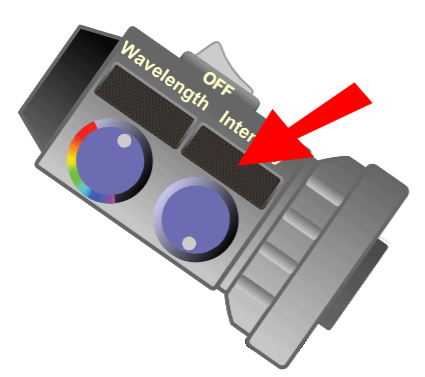
Monochromatic Light Source: This instrument produces a monochromatic light beam of a defined wavelength that hits the cathode plate inside the vacuum tube.

ON/OFF switch: This is used to turn on or off the light source.

Wavelength knob: You can rotate this knob to vary the wavelength of the light beam.
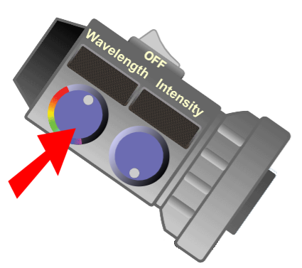
Wavelength display: This shows the value of the wavelength of the light beam in nanometers.

Intensity knob: You can rotate this knob to vary the intensity of the light beam.

Intensity display: This shows the value of the intensity of the light beam as a percentage of a reference maximum value.
Ammeter
Ammeter: This instrument measures the intensity of the photocurrent (the electric current traversing the vacuum tube).

Display: This shows the value of the intensity of the current in microamperes or milliamperes.
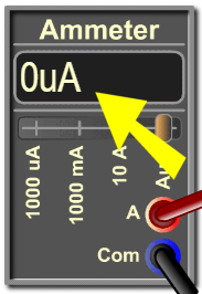
Terminals: These are the terminals of the ammeter (A-terminal and COM-terminal).

Scales: The default scale is automatic (Auto), which automatically switches between µA, mA, and A depending on the magnitude of the measured current.

Vacuum Tube
Vacuum tube: This is the instrument where the photoelectric effect takes place.
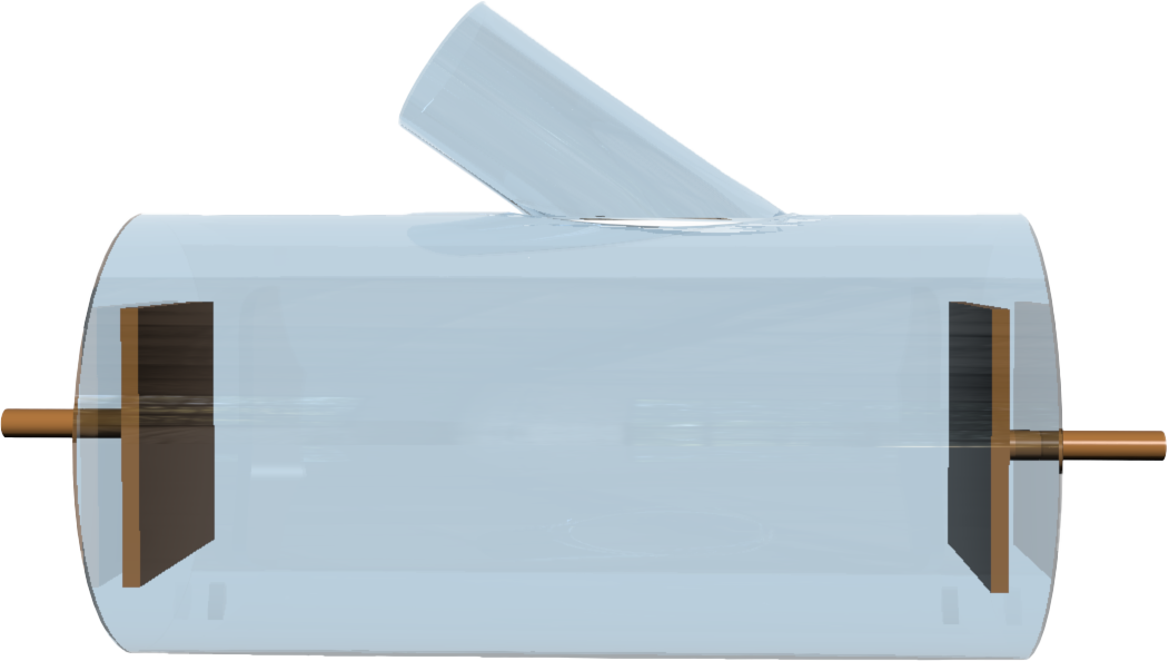
Light beam: The light beam in the inclined branch hits the cathode. The light beam can be modeled as a beam of photons each of energy that depends on the corresponding wavelength of the light beam.

Cathode and Anode: The cathode is connected to the negative terminal of the power supply, and the anode is connected to the positive terminal of the power supply.
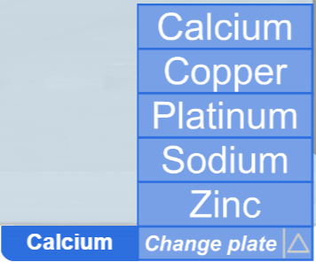
Cathode plate: On the cathode, there is a plate made up of an element of a relatively small work function. The elements used in this experiment are Calcium, Copper, Platinum, Sodium, and Zinc.

Photoelectron emission: For wavelengths smaller than a certain limit, the photons of the beam that are absorbed by the electrons of the surface of the plate give enough energy to the electrons to overstep the work function and fly with some kinetic energy.
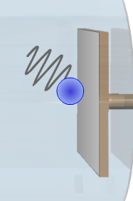
Photocurrent: If this energy is enough to make electrons reach the other plate and be captured by it, then an electric current (called photocurrent) is established between the plates.

Visualization Options
Visualize photons and electrons: Tick this check button to visualize a sample of photons of the light beam and the electrons they release from the plate they hit. Note that not all the released electrons are ejected with the same kinetic energy. The kinetic energy of the emitted electrons ranges between zero and a maximum value that depends on the wavelength of the incident photon and the work function of the material of the plate. Moreover, some photons may not release electrons because they happened to not be absorbed by electrons.

Important caveat: The photons and electrons shown here are only for educational purposes. They are animated to illustrate and explain the process that takes place in the photoelectric effect. These particles are not visible in the experiment. Also, the speed and the number of the photons and electrons shown here are not to scale. They are animated at speeds comfortable to the eye to illustrate the concepts of the experiment.
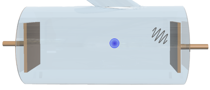
Plate Selection
Change plate menu: Click on this menu to open it and choose among five elements with built-in predefined data. By default, the chosen element is calcium.
Graph
Graph: This is where the variations of some measured physical quantities with respect to other measured physical quantities are plotted.

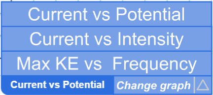
There are three types of graphs available:
Current vs Potential: Plots the variations of the photocurrent as a function of the voltage across the plates. The plotting happens as you vary the voltage generated by the power supply.
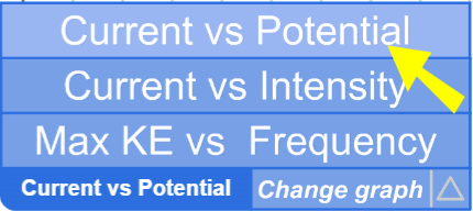
Current vs Intensity: Plots the variations of the photocurrent as a function of the intensity of the monochromatic beam hitting the plate. The plotting happens as you vary the intensity of the light beam.

Maximum Kinetic Energy vs Frequency: Plots the variations of the maximum kinetic energy of the photoelectrons as a function of the frequency of the monochromatic beam. The plotting happens as you vary the wavelength of the light beam (and hence its frequency).

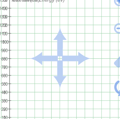
Note that you can drag the graph in all directions to view specific areas outside the frame of the graph.
Graph change menu: Click on this menu to open it and choose among three types of graphs: Current vs Potential, Current vs Intensity, and Maximum Kinetic Energy vs Frequency. By default, the chosen graph is Current vs Potential.
Graph control tools: These are Zoom In, Zoom Out, Clear, and Reset.

Zoom In: Click on this button to zoom in on the graph.

Zoom Out: Click on this button to zoom out of the graph.

Clear: Click on this button to erase all the traces if you want to start a new clean plotting.

Reset: Click on this button to reset the graph to its initial scale and position (without clearing the plotting).

Conclusion
This free online simulation is the most comprehensive and informative among the currently available simulations on the internet. The design emulates an engaging lab environment with a plethora of interactive elements. This enables the student to master a variety of learning objectives and competencies. It assists the teacher and the lab instructor in introducing the concept with an active approach and in blended learning. The simulation is coded with the latest HTML5/JavaScript web tools.